
TL;DR
Render infinitely sharp and anti-aliased SDF by using adaptive sharpening. The sharpening value is calculated from the area that is formed by the Jacobian Matrix of the UV coordinate.
Web Demo
🖱 LMB: Rotate Camera, MW: Zoom, RMB: Pan Camera
Teapot model downloaded from Morgan McGuire’s Computer Graphics Archive
Intro
Signed Distance Field Recap
A Signed Distance Field (SDF) describes a shape by the distance to its closest feature at a given point. A simple example, a wo-dimensional circle, can be described mathematically as:
float circleSdf2d(vec2 samplePosition, vec2 circlePosition, float circleRadius){
  return length(samplePosition - circlePosition) - circleRadius;
}
To actually draw the circle with this function, we would run it for each pixel (using the sample position as the pixel coordinate). If the distance is smaller than 0, we are inside the circle.
We are not limited to circles. More advanced shapes, such as a star, are also possible. This is demonstrated below. Note that the area with a negative distance is colored red.
Compared to a rasterized image, an SDF can always be sharp, no matter how much you zoom in.
From here on, the possibilities of SDFs are enormous and not limited to 2D. Many demos you find on https://www.shadertoy.com/ are built on top of this idea. A comprehensive list can be found here: http://iquilezles.org/articles/distfunctions2d/.
In this article, I will only look into rendering SDFs as simple masks. You can also use gradients, simply by multiplying the final sharpening value we are caluclating here.
Signed Distance Fields And Textures
For many real-time applications, using a zoo of mathematical functions every frame may be too expensive or otherwise unpractical. For example, rendering text with SDFs is a very nice thing to have, given its always-sharp quality. But the glyphs of a font may consist of many individual curves, making it too expensive to calculate every frame. Or take a hand-drawn mask, for example: it can’t even be properly expressed as an SDF.
The solution here is to store the SDF in a texture. This was used by Valve since back in 2007. The most primitive shader snippet that renders such an SDF from a texture may look like this:
half SampleSDFMask(texture2D _SDFTexture, float2 uv) {
	half sdf_raw = tex2D(_SDFTexture, i.uv);		// sample
	half mask = saturate(sdf_raw * 2.0 - 1.0);	// unpack from [0, 1] to [-1, 1] and clamp. (Assuming an area of 1.0 / size-per-texel)
	return mask;
}
So in practice, we just increase the contrast of the texture and call it done. For different scaling factors, you may simply use different unpacking or sharpening factors. And that’s just fine if you render something where each texel ends up at exactly one pixel on the screen. Or, in other words, the area that a single rendered pixel covers is constant.
SDF Textures in 3D
If you want to use an SDF as a texture in 3D, things get tricky, as SDFs can become too crisp in the distance or not sharp enough close up.
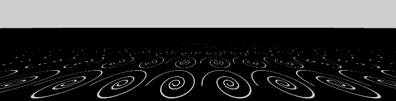
A signed distance field texture that aliases. Notice how the pattern dissolves in the distance.
This is because the distance between two pixels on our SDF-Texture is always constant when viewed in 2D. It is not the same once that texture gets mapped on any 3D surface, due to the perspective transformation. Therefore, we need to know the distance between two texels after the perspective transformation has taken place.
But how do we calculate that distance?
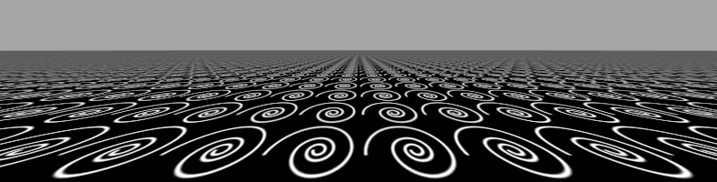
A signed distance field texture that doesn’t alias, using the technique we will develop. Notice how the pattern remains visible in the distance.
Mipmapping
Let’s step back a bit from our problem and look at a problem that is similar to ours, but already well fixed: texture aliasing.
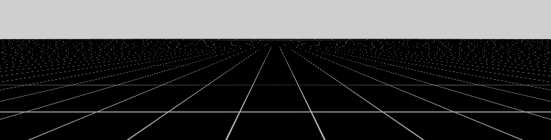
A grid texture without Mipmaps. Notice how the lines of the grid get incomplete at a distance.
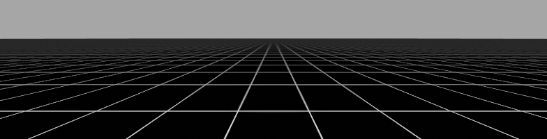
A grid texture with mipmaps. Notice how the lines of the grid remain intact.
When simply mapping a texture onto a 3D surface, chances are high that we will introduce aliasing. That means we are skipping over information, because we are sampling (with the camera) at a lower frequency than the information is available (the texture). This leads to a somewhat noisy and unusable image. Even small movements with the camera will introduce unpleasant noise.
Of course unpleasant is subjective, many retro-esque 3D games use aliasing as part of their visual identity.
The solution to the problem is to have multiple downsized versions of the texture in question. Each mipmap is half the size of the previous mipmap, so that each texel can be seen as a “summary” of four pixels from the larger version.
An image and the corresponding mipmaps on the right side. From Wikipedia
There is a hidden art on how the process of downsampling is done, mainly involving the use of different filter kernels, such as Box, Gaussian or Mitchell. Each of them will give different results, but usually Box is not preferred.
Now, we sample a texture through a shader, say by tex2D(_Texture, uvCoordinate), through some magic, the GPU knows exactly what mipmap to use, so that it never skips over texels or displays a too blurry version. We can kinda guess that it has something to do with the viewing angle and viewing distance, but the solution is much more fun. 😉
The Screen Space Derivative
The main part of that magic is actually the screen space derivative, a handy and special feature of any modern GPU. Instead of trying to guess the area from any viewing angle or distance, we simply use the screen space derivative to get the rate of change of the UV coordinate, with respect to the screen.
In fact, the GPU itself doesn’t even have much of a concept of what viewing angle or viewing distance is. The information to calculate this may not even be supplied in the first place. (Think of what should happen to a mesh without normals to calculate a viewing angle.) By the way if you have access to this information, check out the Dynamic Dilation section in the white paper of the Slug Font Rendering library. You could use the given formula to calculate the derivatives on a per-vertex level.
This is also the reason why even a triangle that is just 1x1 pixels large still generates workload for 2x2 pixels. Even for that single pixel, the GPU needs to know the derivatives. This is a problem with highly detailed meshes and commonly known as quad overdraw.
While for tex2D() this happens under the hood, since Shader Model 3.0 (in DirectX lingo), you are able to get the derivatives for any variable you want, via the HLSL functions ddx() and ddy().
Using ddx(MyUvCoordinate) will give you the rate of change of MyUvCoordinate on the X-axis of the screen and ddy(MyUvCoordinate) for the Y-axis. Getting the screen space derivative for any constant value, let’s say ddx(42), will always give you always 0, as 42 is constant and never changes over the course of the screen.
The following video may give you an idea of how this looks:
Note that I'm showing the length/magnitude ("| |") of the derivative in the video for better illustration.The fragment shader for the left and middle quad.
float4 frag(VertexInput input) : SV_Target0{
 return length(ddx(input.uv)); // ddy for middle
}
The Pixel Footprint
The screen space derivatives alone don’t tell us much, so let’s focus on how we get something useful out of them. For better understanding, let’s introduce the concept of the pixel footprint. This refers to the area that an individual pixel sees.
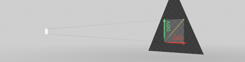
ddX and ddY, displayed as vectors projected onto a triangle. Anisotropic diameter in yellow. The white square represents a single pixel.
We can treat the X and Y screen space derivatives (ddx and ddy) as vectors that span a parallelogram.
While the pixel footprint is not a parallelogram, it is an approximation that works very well most of the time.
We can use this fact to calculate the area, diameter and longest side of the pixel footprint. For mipmaps, it is going to be the longest side, for our SDF the diameter, more on that later.
I don’t know why the longest side is used for mip mapping for sure, but I assume that, since it is the most conservative value, even with heavily distorted UVs it wouldn’t introduce aliasing.
Equipped with this knowledge, we can now calculate the mipmap index ourselves.
float GetMipMapLevel(float2 uv, float2 texel_size) {
    // convert UV space [0,1] to texel space [0..axis_size].
    float2 dx_uv = ddx(uv) * texel_size;
    float2 dy_uv = ddy(uv) * texel_size;

    // calculate the squared length of the longest axis.
    float longest_side = max(dot(dx_uv, dx_uv), dot(dy_uv, dy_uv));

    // take the square root of the squared-longest-side and use log2 to get the according mip-map index.
    // Log2 is used because mip-maps are index by thier base to the power-of-two.
    // Note that: 0.5 * log2(longest_side) == log2(sqrt(longest_side))
    return 0.5 * log2(longest_side);
}
You can also look at the reference here: the OpenGL 4.2 specifications. Look at equation 3.21. Note that, for some reasons, the formula doesn’t take the texture resolution into account. It will not work out of the box when you use it in shader code. This is “fixed” in the above version. If you know more about why it is like this in the specs, I’d be happy to hear!
Filtering The SDF
For the SDF, however, we are not interested in the mip-map level.
Remember, our initial goal was to calculate the distance between two texels after the perspective transformation. Instead of the longest side as for mip-maps we are going to use the diameter of the pixel footprints area this.
In my tests using the diameter had better sharpening and less aliasing, especially on step viewing angles.
To calculate the area first, we can use the Jacobian Matrix, a matrix that is built by the partial derivatives, in our case, the screen space derivatives of the UV. In HLSL, it is built as float2x2 uvJacobian = float2x2(ddx(uv), ddy(uv)). If we now calculate the determinant, we get a value that essentially indicates the “space distortion” of a matrix. In the case of the 2D Jacobian Matrix, this is identical to calculating the area of a parallelogram. Finally, after the taking the square root of the area, we got what we needed.
This animation may help visualize what is happening with the diameter under different viewing conditions.
If we multiply the pixel footprint area by the number of texels (the texture resolution), we get the area in texel space that the pixel covers. That means that if this value is 1.0, we have exactly one texel under the pixel. A value larger than 1.0 means more than one texel per pixel, and vice versa.
Putting it together, we get:
float FilterSdfTextureExact(float sdf, float2 uvCoordinate, float2 textureSize) {
    // Calculate the derivative of the UV coordinate and build the jacobian-matrix from it.
    float2x2 pixelFootprint = half2x2(ddx(uvCoordinate), ddy(uvCoordinate));
    // Calculate the area under the pixel.
    // Note the use of abs(), because the area may be negative.
    float pixelFootprintDiameterSqr = abs(determinant(pixelFootprint));
    // Multiply by texture size.
    pixelFootprintDiameterSqr *= textureSize.x * textureSize.y ;
    // Compute the diameter.
    float pixelFootprintDiameter = sqrt(pixelFootprintDiameterSqr);
    // Clamp the filter width to [0, 1] so we won't overfilter, which fades the texture into grey
    pixelFootprintDiameter = saturate(pixelFootprintDiameter) ;
    return saturate(inverseLerp(-pixelFootprintDiameter, pixelFootprintDiameter, sdf));
}
Bonus: Why Not Just Use fwidth() Directly For Filtering?
Some resources may point out the usage of fwidth() directly, as in
half SampleSDFMask(texture2D _SDFTexture, float2 uv) {
	half sdf_raw = tex2D(_SDFTexture, i.uv);		// sample
  half mask_fwidth = fwidth(mask);
	half mask = saturate((sdf_raw * 2.0 - 1.0) / mask_fwidth);
	return mask;
}
As a recap, fwidth() is defined as
abs(ddx(p)) + abs(ddy(p)).
So instead of taking the derivative of the UV, we take the sampled SDF value directly.
This is not optimal for two reasons:
- It will introduce aliasing, since the “sharpening value” is calculated for 2x2 pixel blocks and not per-pixel.
- It creates a hidden dependency between the pixels, because in order to know the value of
mask_fwidth, all four pixels need to know the value ofmaskfirst.